 Geethaa Srinivasan
Machine Learning is classified as Supervised and Unsupervised Machine Learning. Regression and Classification come under supervised Machine Learning. In this post, we will see Regression with an example, the iterative process involved in supervised machine learning and evaluation metrics.
Introduction
Regression models predict numeric label values based on features and known labels in the training data. The process of training the regression model involves training, evaluation, and refining of the model.
The steps involved in an iterative process of supervised machine learning
- Split the training data and hold a subset of data to validate the model.
- Use a linear regression algorithm to fit the training data to the function.
- Use held-back validation data to predict labels for features.
- First, compare the actual labels with the model-predicted labels and calculate the aggregate difference between them to calculate the metrics.
The process is repeated with different algorithms and parameters until we achieve the desired predictive accuracy.
Example
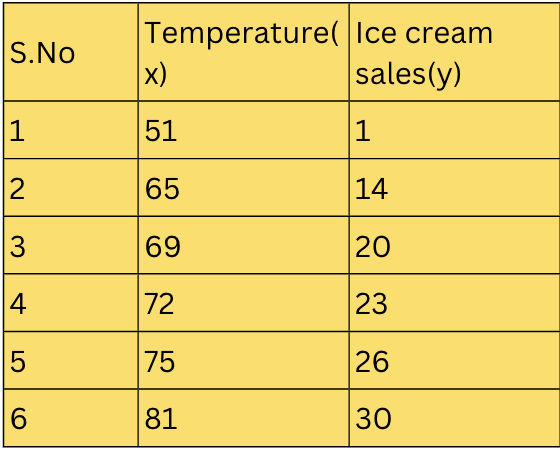
We train the model to predict label (y) based on a single feature(X), in most cases, there can be multiple features.
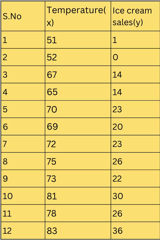
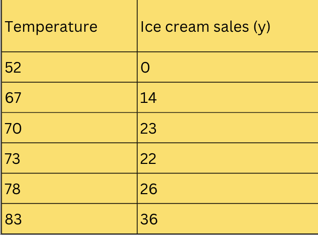
The table below shows historic data of ice cream sales as an example with maximum temperature as feature (x) and ice cream sales as label(y).
For the video tutorial check Master Regression: Training Models SImplified
Training a regression model
To find the relation between x and y we plot a graph
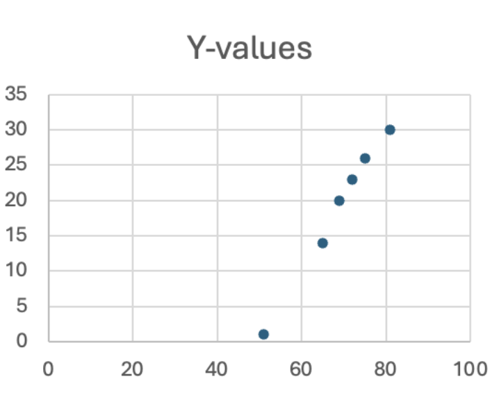
We apply algorithms such as the Linear regression algorithm to fit the training data to a function. The above graph represents a function in which the slope describes how to calculate y for different values of x.
From the above graph, we can understand that at
x=50, y=0
x=55, y=5 from this we can infer that the increase of x up by 5 units increases y by 5. From this, we can express the function as
f(x)=x-50
The above function can predict ice cream sales on a particular day. For example, if tomorrow’s temperature is 77 degrees we can predict ice cream sales on that day using the function
f(x)=77-50 =>27 ice creams.
Evaluating Regression Model
To evaluate the model, the data that is held back is used.
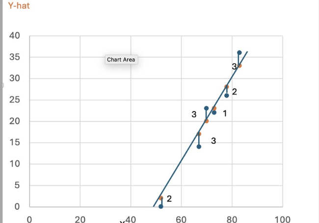
We use the function, predict the label for different features, compare the predicted values with actual values, and plot the graph.
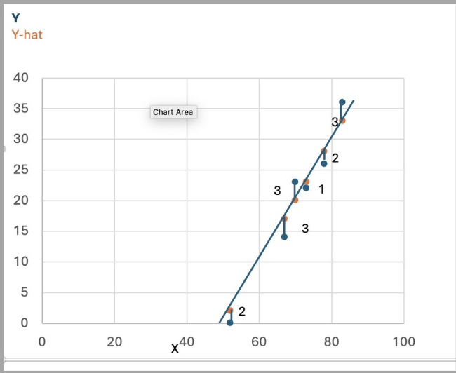
From the above graph, we can infer the variance between the predicted and the actual value.
For the video tutorial check Regression Metrics | MSE, MAE & RMSE | R-squared
Regression Evaluation Metrics
To evaluate the regression models, we use some common metrics calculated using the difference between the predicted and the actual value.
Mean Absolute Error(MAE)
How much value each prediction was wrong irrespective of +ve or -ve difference is referred to as the Mean Absolute Error. From the graph, we can calculate MAE for ice cream sales example as
(2+3+3+1+2+3)/6 =>2.33
Mean Squared Error(MSE)
To choose a model that produces fewer errors we need to amplify larger errors by squaring individual errors and calculate the mean of the squared values referred to as Mean Squared Error(MSE).
MSE for ice cream sales example => 2,3,3,1,2,3 =>
4+9+9+1+4+9=>36/6=>6
Root Mean Squared Error(RMSE)
The MSE metric just provides the error value and does not provide the information about the number of ice creams mispredicted since it squares the value. For this, we need a metric that tells how many were mispredicted, hence we calculate Root Mean Squared Error (RMSE).
For ice cream sales, √6 =>2.45
Coefficient of Determination (R2)
The Coefficient of Determination, R-squared, R2 is a metric that calculates the proportion of variance in the result as opposed to the anomalous aspect of the validation data.
It compares the sum of squared differences between predicted and actual labels with the sum of squared differences between the actual and the mean of actual label values, R2 = 1- ∑(y-ŷ)2 ÷ ∑(y-ȳ)2
The result lies between 0 to 1, closer to one better is the model. For ice cream sales R-squared is 0.95
Iterative Training
The iterative process of training and evaluation is repeated to determine the best model that is suitable for a specific scenario,
But with slight variations in
- Feature selection and preparation
- Algorithm selection
- Algorithm parameters (numeric settings to control algorithm behavior, called hyperparameters to differentiate them from the x and y parameters).