 Vinodh Ramu
Part of the “Understanding LLM from Scratch” collection — standalone posts unpacking how LLMs actually work, written as I learn.
Multilingual embeddings are the mechanism that lets a language model read “5 Mani ku alarm vai” — a sentence that blends Tamil and English — and understand it without a translation step. This post traces how raw token IDs become meaning, why languages share the same geometric space inside a model, and what that means for anyone building AI systems for real-world users.
It Started with My Daughter
My daughter was doing her homework one evening. Mid-way through, without looking up from her books, she called out to Gemini on her iPad:
“5 Mani ku alarm vai”
Tamil for “Set an alarm at 5 o’clock.” Not pure Tamil — a numeral, an English loanword (alarm), and three Tamil words, all in one breath. No pause. No switching to English for the device’s benefit.
Gemini set the alarm.
No confusion. It didn’t ask her to repeat herself. No falling back to a generic error. It understood exactly what she meant — set a reminder for when it was time to stop studying.
She went straight back to her homework. She didn’t think twice about it. Meanwhile, I was sitting nearby, and I did.
The Gap the Last Post Left Open
In the previous post, we learned that text becomes token IDs before a model ever sees it. Byte Pair Encoding splits the input into subword pieces and maps each one to an integer. For her spoken sentence — transcribed to text — a tokenizer would produce something like:
import tiktoken
enc = tiktoken.get_encoding("cl100k_base")

text = "5 Mani ku alarm vai"
tokens = enc.encode(text)
decoded = [enc.decode([t]) for t in tokens]

print(f"Token IDs: {tokens}")
print(f"Decoded:   {decoded}")
# Token IDs: [20, 31562, 18375, 15435, 348, 990]
# Decoded:   ['5', ' Man', 'i', ' ku', ' alarm', ' vai']
So the model receives: [20, 31562, 18375, 15435, 348, 990]
Six integers. That’s it.
Now here’s the question that kept me up: how does a list of integers become understanding?
The answer is multilingual embeddings.
From Token IDs to Embedding Vectors
A token ID is just an index into a lookup table. Every model has an embedding matrix — a large table where row n is the vector representation of token n. When token ID 348 ( alarm) enters the model, it looks up row 348 in that table and retrieves a vector of floating-point numbers.
For GPT-sized models that vector is 768 to 12,288 numbers long. For smaller models, shorter. But the principle is the same:
# Conceptual illustration — not runnable as-is
# Assume an embedding matrix E of shape [vocab_size, embedding_dim]

token_id = 348          # ' alarm'
embedding_dim = 768

vector = E[token_id]    # shape: (768,)
# → array([-0.023,  0.417,  0.089, -0.312, ..., 0.201])  # 768 numbers
One token. 768 numbers. Each number is a coordinate in a 768-dimensional space.
That sounds abstract. So before we go further, let me make it concrete.
What a Vector Actually Represents
Forget 768 dimensions for a moment. Imagine you could describe every word using just two numbers:
- Axis 1: how “living” the thing is (0 = inanimate, 1 = alive)
- Axis 2: how “large” it is (0 = tiny, 1 = enormous)
You could then plot words as points on a 2D grid:
             large
               │
    elephant ──┼── truck
               │
alive ─────────┼───────── inanimate
               │
    cat ───────┼── phone
               │
             small
In this toy space, cat and elephant are close on the “alive” axis. truck and elephant are close on the “large” axis. cat and truck are far apart on both.
Real embeddings do the same thing — but with 768 axes instead of 2, and the axes are not hand-labelled. The model learns what those axes should represent during training, entirely from the patterns in text. Some axes end up encoding concepts like “living vs. inanimate”, others encode “positive vs. negative sentiment”, “formal vs. informal register”, and hundreds of other dimensions the model discovered were useful for predicting the next word.
The vector for alarm has a position in that 768-dimensional space. So does Mani. Whether they end up near each other depends entirely on what the model was trained on.
The Geometry of Meaning
The key insight is not that embeddings exist — it’s where they land.
Specifically, during training, the model adjusts every vector in the embedding matrix to minimise prediction error. Words that appear in similar contexts get pulled toward similar positions. Not because anyone wrote a rule — because it minimises loss.
The result is that the embedding space has geometric structure that mirrors semantic structure.
Let me show this concretely. Using the sentence-transformers library — the same one I mentioned in the last post as the embedding engine behind our vector search tool:
from sentence_transformers import SentenceTransformer
from sklearn.metrics.pairwise import cosine_similarity
import numpy as np

model = SentenceTransformer("all-MiniLM-L6-v2")

words = ["dog", "cat", "car", "truck"]
embeddings = model.encode(words)

# Compute pairwise cosine similarities
for i, w1 in enumerate(words):
    for j, w2 in enumerate(words):
        if j > i:
            sim = cosine_similarity([embeddings[i]], [embeddings[j]])[0][0]
            print(f"{w1:8} ↔ {w2:8}  similarity: {sim:.3f}")
Sample output:
dog      ↔ cat       similarity: 0.814
dog      ↔ car       similarity: 0.271
dog      ↔ truck     similarity: 0.198
cat      ↔ car       similarity: 0.243
cat      ↔ truck     similarity: 0.179
car      ↔ truck     similarity: 0.782
dog and cat score 0.814 — very close. car and truck score 0.782 — also close. But dog and car score 0.271 — far apart.
No dictionary was consulted. No taxonomy was hardcoded. Instead, the model learned these relationships purely from reading text where dogs and cats appeared together, and cars and trucks appeared together.
Think of it as a neighbourhood map. dog and cat live on the same street. car and truck live a few blocks away in a different part of town. dog and car are in entirely different districts. Nobody drew this map — it emerged from the model asking, millions of times: “given everything I’ve seen, which words tend to appear near each other?”
This is the foundation on which multilingual understanding is built.
Same Meaning, Different Language — How Multilingual Embeddings Bridge Languages
Here is where it gets interesting.
If you train on enough multilingual text, the same geometric compression happens across languages. The model sees “dog” and “chien” in similar contexts — perhaps in parallel news articles, subtitles, or Wikipedia pages that link English and French versions. Over millions of such co-occurrences, the two vectors get pulled toward the same region.
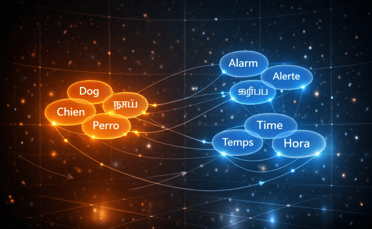
The result is a shared multilingual embedding space — a single coordinate system where tokens from every language live, and where semantic neighbours are neighbours regardless of which language they came from.
Think back to the neighbourhood map. In a monolingual model, dog lives next to cat, puppy, bark, leash. In a multilingual model, its neighbours also include chien (French), perro (Spanish), நாய் (Tamil), Hund (German) — because all of them appeared in similar contexts across the training data. The word changed. The meaning — and therefore the neighbourhood — did not.
      [semantic neighbourhood of "dog"]

   chien (FR) ── dog (EN)
        \           /
         \         /
          [ "dog" ]
         /         \
        /           \
  நாய் (TA) ── perro (ES)
The tightness of that cluster depends entirely on how much multilingual data the model trained on. Which is exactly what our experiments will show.
But not all multilingual models are created equal. Let me run the same experiment twice — with two different models — and show you what that difference actually looks like.
Experiment A — paraphrase-multilingual-MiniLM-L12-v2
from sentence_transformers import SentenceTransformer
from sklearn.metrics.pairwise import cosine_similarity

model = SentenceTransformer("paraphrase-multilingual-MiniLM-L12-v2")

# "dog" in English, French, Tamil, Spanish
words = ["dog", "chien", "நாய்", "perro"]
labels = ["dog (EN)", "chien (FR)", "நாய் (TA)", "perro (ES)"]

embeddings = model.encode(words)

for i, l1 in enumerate(labels):
    for j, l2 in enumerate(labels):
        if j > i:
            sim = cosine_similarity([embeddings[i]], [embeddings[j]])[0][0]
            print(f"{l1:15} ↔ {l2:15}  similarity: {sim:.3f}")
Output:
dog (EN)        ↔ chien (FR)       similarity: 0.980
dog (EN)        ↔ நாய் (TA)        similarity: 0.504
dog (EN)        ↔ perro (ES)       similarity: 0.990
chien (FR)      ↔ நாய் (TA)        similarity: 0.614
chien (FR)      ↔ perro (ES)       similarity: 0.989
நாய் (TA)        ↔ perro (ES)       similarity: 0.533
Two stories in one output. English, French, and Spanish form a tight cluster at 0.98–0.99 — the model treats them as near-identical in meaning. Tamil is the outlier: 0.50–0.61 against the other three. The model has learned something about Tamil (0.5 is well above random), but the alignment is weak.
This is not a Tamil problem. It is a training data problem. paraphrase-multilingual-MiniLM-L12-v2 was trained with stronger coverage of European languages than South Asian ones. The embedding space reflects that imbalance directly.
So I asked the natural follow-up question: what happens if I use a model specifically built for broader language coverage?
Experiment B — LaBSE (Language-Agnostic BERT Sentence Embeddings)
LaBSE is a model developed at Google, trained on parallel corpora across 109 languages with explicit coverage of Indian languages including Tamil. Same experiment, different model:
from sentence_transformers import SentenceTransformer
from sklearn.metrics.pairwise import cosine_similarity

model = SentenceTransformer("sentence-transformers/LaBSE")

words = ["dog", "chien", "நாய்", "perro"]
labels = ["dog (EN)", "chien (FR)", "நாய் (TA)", "perro (ES)"]

embeddings = model.encode(words)

for i, l1 in enumerate(labels):
    for j, l2 in enumerate(labels):
        if j > i:
            sim = cosine_similarity([embeddings[i]], [embeddings[j]])[0][0]
            print(f"{l1:15} ↔ {l2:15}  similarity: {sim:.3f}")
Output:
dog (EN)        ↔ chien (FR)       similarity: 0.965
dog (EN)        ↔ நாய் (TA)        similarity: 0.962
dog (EN)        ↔ perro (ES)       similarity: 0.942
chien (FR)      ↔ நாய் (TA)        similarity: 0.950
chien (FR)      ↔ perro (ES)       similarity: 0.920
நாய் (TA)        ↔ perro (ES)       similarity: 0.946
Tamil is now fully in the cluster — 0.94–0.96 across the board, on par with French and Spanish. The same word, the same concept, the same sentence. The only thing that changed was the model.
This is the result I was looking for when I first wondered how “5 Mani ku alarm vai” worked. The answer isn’t just “multilingual embeddings” — it’s which multilingual embedding model, trained on which languages, with how much data.
How Training Pulls Languages Together
This alignment isn’t magic — it has a mechanism.
Consequently, Tamil had weaker alignment in Experiment A — Tamil parallel data is less abundant than French or Spanish parallel data in that model’s training set. Moreover, LaBSE was specifically built to address this — its training included broader multilingual parallel data with deliberate coverage of Indian languages, which is why Tamil snapped into the same cluster in Experiment B.
Additionally, even without parallel data, multilingual models benefit from shared subword tokens. Recall from the BPE post: punctuation, numbers, and many proper nouns tokenize identically across languages. Those shared anchors act as alignment pins in the embedding space, giving the model footholds to connect different language clusters.
Back to “5 Mani ku alarm vai”
Now we have everything we need to trace what actually happened that evening.
When my daughter spoke to Gemini on her iPad and the speech-to-text layer transcribed “5 Mani ku alarm vai”, here is the full pipeline the model ran:
Step 1 — Tokenization (BPE) The sentence splits into subword tokens. Tamil tokens like Mani and vai become their own token IDs. The English token alarm gets its usual ID. The numeral 5 gets its usual ID.
Step 2 — Embedding lookup Next, each token ID is replaced by its embedding vector. Here is where multilingual embeddings do their work: the Tamil token for `Mani` (மணி, meaning “o’clock” / “time”) has been pulled — during training — toward the same neighbourhood as `hour`, `o’clock`, and `time` in English. Not because of a dictionary. Because they appeared in similar contexts across millions of documents.
Step 3 — Contextual reasoning (Transformer) From there, the model passes all the vectors through its attention layers (that’s the next post). Each token attends to every other token. The numeral `5`, sitting next to `Mani`, reinforces the “time” interpretation. `alarm` confirms the task type. `vai` (Tamil for “set” / “put”) pushes toward an action intent.
Step 4 — Output Finally, the model generates a response consistent with setting a 5 o’clock alarm — in English, because that is the dominant output language in its training distribution.
No translation module. No language detection step. No special Tamil handler. My daughter just talked to a device the way she talks at home — and the shared geometric space did the rest.
Multilingual Embeddings and Emergent Translation
This is what I find most striking about multilingual embeddings — they produce translation as a side-effect, not a feature.
The model was never trained to translate Tamil to English. It was trained to predict the next token accurately on a large multilingual corpus. As a consequence of doing that well, it learned that tokens meaning the same thing in different languages are interchangeable in context. Translation falls out of that as emergent behaviour.
This is why multilingual embeddings are such a powerful primitive. You do not need to anticipate every language combination your users might produce. As long as the model trained on both languages, the shared embedding space handles the bridge automatically.
Why This Matters — Real Consequences of Multilingual Embeddings
Understanding how multilingual embeddings work changes the way you think about building AI systems.
1. Cross-lingual search works out of the box
Because embeddings encode meaning rather than words, you can query in one language and retrieve documents in another. A user searching “நாய் உணவு” (dog food in Tamil) will surface results written in English about dog food — not because the search engine translated the query, but because the query vector and the document vectors land in the same neighbourhood. This is how multilingual vector search works in systems like the pgvector tool we built in the agents series.
2. Inclusive assistants without special handling
However, not all multilingual models cover all languages equally. As we saw, `paraphrase-multilingual-MiniLM-L12-v2` (118M parameters) gave Tamil weak alignment while LaBSE (471M parameters) fully resolved it — at roughly 4× the model size. In fact, choosing the wrong multilingual model for your language set doesn’t just waste compute; it silently degrades quality for the users you were trying to include. Knowing *why* different models produce different alignment helps you make that choice deliberately rather than defaulting to whatever the tutorial used.
4. Low-resource languages get a compounding disadvantage
Recall from the BPE post that rare subwords get fewer merge operations — so low-resource language tokens tend to be shorter, more fragmented pieces. Those fragments also appear less frequently in training data, which means the embedding model has fewer co-occurrence signals to align them with equivalents in other languages. We saw this directly: Tamil scored 0.50–0.61 with paraphrase-multilingual-MiniLM-L12-v2, compared to 0.98–0.99 for the European languages. Switching to LaBSE — a model trained with broader multilingual coverage — brought Tamil to 0.94–0.96. The gap is closeable, but only by choosing a model that was deliberately trained to close it.
The core insight: The model doesn’t translate. It never needs to. When training on multilingual corpora pulls “alarm” and “Mani” into the same neighbourhood, understanding one automatically means understanding the other — regardless of which language the user happens to be speaking in at that moment.
Try It Yourself
- Verify the classic word analogy: Encode
"king","queen","man","woman"with a multilingual model. Computeking − man + woman. Is the resulting vector closest to"queen"? This is the classic word2vec demonstration — does it still hold in sentence-transformer space? - Test your own code-switching sentence: Write a sentence that mixes your native language with English — the way you’d actually type it to a friend. Feed it to an AI assistant and to the embedding model. Does the model understand it? Does the embedding land near what you expected?
- Find a false friend across languages: The Spanish word “embarazada” means pregnant, not embarrassed. Encode both and check their cosine similarity. Are false friends close in embedding space, or has the model learned to separate them based on context?
- Compare a high-resource vs. low-resource language: Encode “I love coffee” in English, French, and a low-resource language like Swahili or Tagalog. Which translation is closest to the English embedding? Does the resource level of the language predict the alignment quality?
- Reproduce the two-model contrast: Run Experiments A and B from this post with a language you speak. Does the lower-coverage model show the same outlier pattern for your language that we saw with Tamil? Does switching to LaBSE close the gap? The answer tells you which model you should actually be using in production.
I’m learning LLMs from scratch — reading, implementing, and writing as I go. Next up: how the model uses these vectors — the attention mechanism, and why a single idea called “self-attention” changed everything.